A Librarian’s Guide to AI in Academic Search Tools
As Katina covers the integration of AI into academic search tools and other library products, this guide offers useful background information on the technology.

As Katina covers the integration of AI into academic search tools and other library products, this guide offers useful background information on the technology.

This guide provides an overview of these subjects:
LLMs are advanced AI systems trained on vast amounts of text data, enabling them to both understand text and generate human-like summaries and answers to questions. Popular LLMs include proprietary models like OpenAI’s GPT, Anthropic’s Claude, Google’s Gemini, and open-source models like Meta’s Llama and DeepSeek.
(Note: Modern LLMs powered by Transformer architectures reach or approach near human-level scores in many prominent natural language benchmarks in tasks such as summarization, sentiment analysis. However, philosophers and linguists still argue whether such models have genuine “understanding” in the same way as humans do, as opposed to merely being very sophisticated statistical pattern-matchers (Bender et al., 2021; Bender & Koller, 2020). I’ll use “understand” and similar terms throughout this guide but take no position in the larger debate.)
The term “retrieval augmented generation,” or RAG, was first coined in a 2020 paper (Lewis et al., 2021). RAG is popularly used in academic search systems to blend search with large language models. A typical RAG system will not just generate an answer to your query but will provide citations to documents that support the answer (see Figure 1 for a sample answer). But how does it do so?

Think about the difference between a closed-book exam (where you rely only on memory) and an open-book exam (where you look things up before answering). RAG is like an open-book exam for an AI system.
Figure 2 illustrates how RAG typically works in academic AI search engines, including Primo Research Assistant, Web of Science Research Assistant, and Scopus AI.
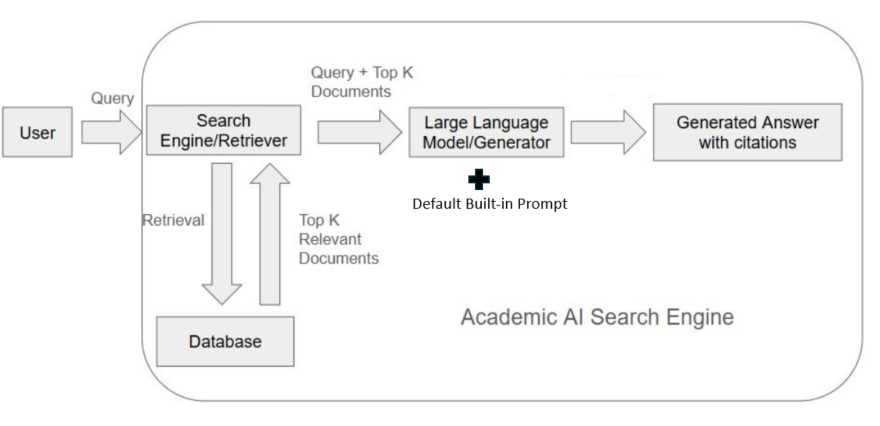 FIGURE 2
Here’s a simplified explanation:
1. You Ask: You type your research question into the tool.
2. The System Searches (Retrieval): Instead of answering immediately, the tool first searches its specific, trusted academic database (like Primo’s index, Scopus, or Web of Science) for documents related to your question. It picks out the top few results.
3. The System Reads and Writes (Augmented Generation): The LLM then runs a default, built-in prompt to use the information from those specific documents to write a summary answer to your question, including citations that point back to the documents it used.
An example of what this default prompt might look like appears in Figure 3.
 FIGURE 3
What are the advantages of RAG versus just using a LLM directly without search?
Do note that many modern LLMs, like ChatGPT, Gemini, Claude, and Grok, have search/RAG capabilities. However, two things still distinguish them from academic AI search engines: while they can search, they do not always “choose” to search. And they use general web search, e.g. Bing, while academic AI search systems search academic content in scholarly indexes.
Beyond traditional keyword searching, some modern AI tools utilize embedding search, also sometimes known as vector search, neural search, or semantic search. At the core of this approach are “embeddings” or “vectors,” that is, sophisticated numerical representations of key parts of the text (like titles, abstracts, or chunks of full text). Embeddings are essentially long lists of numbers, often with hundreds or even thousands of dimensions (common sizes include 768 or 1536 dimensions), where each dimension represents some aspect of the text’s meaning. The high dimensionality allows these vectors to capture very complex semantic nuances and relationships between concepts.
Embeddings are generated using complex neural network models. State-of-the-art systems typically employ a type of neural network architecture dubbed the “Transformer model” in the seminal 2017 paper “Attention is all you need”(Vaswani et al., 2017), which laid the foundation for popular models used today (e.g. BERT, GPT). These models are trained on massive datasets and excel at understanding the context in which words appear—analyzing surrounding words and sentence structure. This process allows them to encode nuanced meaning, relationships, and context into the high-dimensional vectors, creating a rich mathematical representation of the text’s core concepts.
Embedding search leverages these vector representations. When you submit a query, it is run through an embedding model that converts the query into its own embedding vector to represent the query.
The system then mathematically compares this query vector to the pre-calculated embedding vectors of the documents in the index (which represent the documents). It identifies documents whose vectors are mathematically closest to the query vector within that high-dimensional “meaning space.” This proximity, often calculated using measures like cosine similarity, signifies strong semantic relevance between the query and the document, forming the basis of the search results.
Why do this? The embedding method can overcome the “vocabulary mismatch problem,” where relevant documents are missed because the query terms used do not match. But it is not a silver bullet, and in some situations, is outperformed by keyword search. This is why many systems (for example, Scopus AI) are a hybrid of both methods.
The first popular vector embedding for individual words was Word2Vec, released by Google in 2013 (Mikolov et al., 2013).
The main idea of Word2Vec is that words with similar meanings tend to appear in similar contexts. Word2Vec uses a simple neural network to learn by looking at words that occur near each other in sentences.
The Word2Vec method involves feeding the network sample sentences from the internet and training the network to predict neighboring words for a given word (Skip-gram) or to predict the given word from its neighbours (CBOW). By adjusting the network’s internal weights through many examples, Word2Vec gradually learns numerical representations that capture word meanings.
Google found that once they trained Word2Vec this way over a huge set of data (Google News text, or about 100 billion words), the embeddings (300 dimensions) that were produced seemed to encode semantic meaning. For example, they famously found that the embeddings for king - man + woman ≈ queen (Mikolov et al., 2013).
Today, modern embeddings go beyond the basic neural networks used in Word2Vec, mostly using Transformer-based neural network architectures instead (e.g. BERT).
While Word2Vec is a word-level embedding, the concept of embeddings can be used at different levels of granularity:
Word level: Map individual words to vector embeddings (e.g., Word2Vec, GloVe (Pennington et al., 2014)).
Sentence embeddings: Map words and whole sentences to vector embeddings (e.g., SBERT (Reimers & Gurevych, 2019), Universal Sentence Encoder (Cer et al., 2018)).
Document embeddings: Map whole documents to vector embeddings
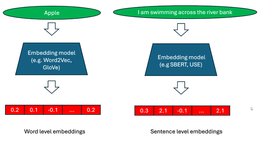 FIGURE 4
Because embeddings are trained using neural networks, they are black boxes: it is almost never possible to interpret what each number means.
In the example below, I ran the words “Apple,” “Orange,” and “Car” individually through a popular OpenAI embedding model named text-embedding-3-small, which has 1,536 dimensions (Open AI, 2024) (Model - OpenAI API, n.d.). Another way to say this is that text in this embedding is represented in 1,536 numbers, or in 1,536-dimensional space.
Here are the first two numbers and the last numbers of the embeddings representing “Apple,” “Orange,” and “Car.”
Dimension | 1 | 2 | … | 1536 |
Apple | 0.0176 | -0.0168 | … | 0.007 |
Orange | -0.0259 | -0.0055 | … | -0.0147 |
Car | 0.0085 | -0.0040 | … | -0.003 |
While it is true that if you run a similarity measure like cosine similarity between the three words, you will find “Apple” is indeed closer (or has higher cosine similarity) to “Orange” compared to “Car,” you will not be able to interpret what each individual number in the embeddings mean.
This problem is compounded if you use sentence-level embeddings, as all the words in the sentence are “squeezed” into one embedding. There are more sophisticated multiple embedding approaches, like ColBERT, that store individual embeddings for each token or word in a text chunk. This improves interpretability.
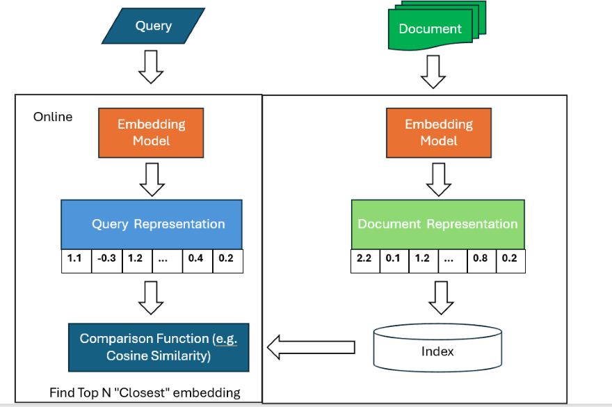 FIGURE 5
Information retrieval needs to be fast. A common way to leverage embeddings is to adopt a “bi-encoder” model (Reimers & Gurevych, 2019). When documents are being indexed, they are run through an embedding model which converts the text in the documents to embeddings that represent the documents, which are then stored in a special index known as a vector store.
When you enter a query, your query is converted in real-time to an embedding using the same embedding model to create a representation of the query. Assuming your RAG model wants to find the top eight results, the query embeddings are compared against the document embeddings by using a comparison function, such as cosine similarity, to find the top eight closest document embeddings.
But imagine if the index has 100 million document embeddings. If you tried to compare the query embedding, or representation, against all 100 million document embeddings, it would take too long.
There are faster methods that can guarantee that you will find the closest document embedding without going through all 100 million documents, but in practice, most embedding search engines use shortcut methods such as “approximate nearest neighbor” (ANN).
While ANN methods are fast, they often lead to searches being less reproducible—that is, the same exact query entered multiple times sometimes results in different documents being retrieved or in documents being retrieved in different orders, even if the index is unchanged.
Faster methods like ANN use “guessing” to approximate results, which may miss some of the true closest documents (Elastic, 2024).
Here’s a rough analogy: imagine a library of one million books indexed by subject headings that cluster similar subjects together. A librarian is asked to find the five books most relevant to “history of trade wars.” Rather than scanning every book she:
Another librarian might choose a different starting point, yielding slightly different results.
This is how approximate nearest neighbor (ANN) search works: the same query can produce varied results depending on the starting point.
Technically, some systems store the “seed,” or starting point, within a session to ensure consistent results, but starting a new session with the same query may trigger the selection of a different starting point, leading to different results.
Searching more thoroughly reduces the chance of missing the true top eight, but the differences are often minor enough that the trade-off in faster speed is worth it.
Implementing embedding search as the primary retrieval method across an entire index can be computationally intensive and costly, often requiring the creation and maintenance of large vector databases to store document embeddings during the pre-indexing phase. A more efficient and cost-effective alternative is to use embedding search for reranking.
This approach works in two stages:
This method leverages the speed of traditional search in the initial filtering and applies the nuanced semantic understanding of embeddings only where it’s most likely to matter—on the most promising candidates. Because the system only needs to calculate the embedding of a small number of documents, it can do so on the fly rather than constructing embeddings of the whole index in advance and storing them in a separate vector database.
Because embedding search and keyword searching have their separate strengths and weaknesses, hybrid searches that combine two or more retrieval systems are common (Cardenas, 2025).
Scopus AI, for example, uses both a keyword Boolean search (with a search strategy generated by LLM) and an embedding search in parallel, combining the top results.
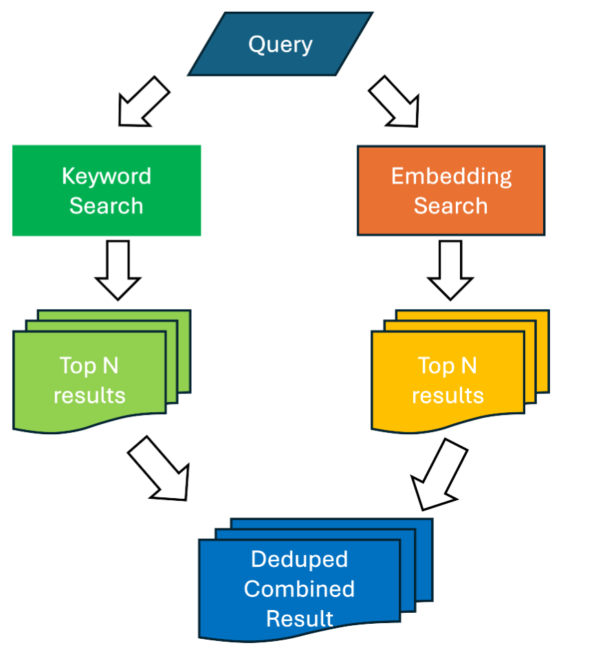 FIGURE 6
Taking this approach, an AI search engine might combine the top 500 results from a keyword search and the top 500 from an embedding search, dedupe the combined result set, and rank them again.
How would it rank the combined result set? One simple yet popular method is reciprocal rank fusion (Cormack et al., 2009). This table shows reciprocal rank fusion in action:
| Rank in algo 1 | Rank in algo 2 | Overall Relevancy Score |
Doc A | 1 | 2 | 1/1 + 1/2 = 1.5 |
Doc B | 5 | 3 | 1/5+1/3 = 0.533 |
Doc C | 10 | 8 | 1/10 + 1/8 = 0.225 |
As the table shows, you just sum the reciprocals of each rank to create an overall ranking.
(In practice, the actual formula for the contribution to RRF is (1/ (k+rank)), where k is typically 60. So, for example, rank 1 contributes (1/(60+1) = 0.0164 instead of 1.K is a damping factor used to reduce the impact of top-ranking positions.)
Besides using simple methods like RRF to combine results, it is also common to run the combined results set from the hybrid search through a reranker.
A reranker is a more powerful algorithm that is very accurate but too slow to run over all the documents in your index. There are many types of rerankers—this blog post offers a detailed but still accessible discussion (Clavié, 2024)—but I will focus on two here.
First let’s discuss the cross-encoder model.
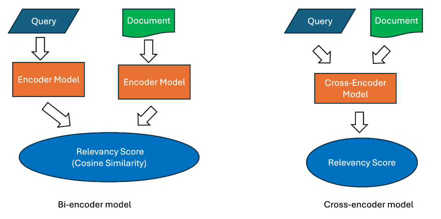 FIGURE 7
We already met the bi-encoder model, where we convert the query and documents separately by running them through an embedding model, typically a Transformer-based encoder model that encodes queries and documents into embeddings and then compares the two embeddings using a similarity measure like cosine similarity. The bi-encoder model has the advantage of being able to convert the documents into embeddings “in advance.”
But the cross-encoder model is even more powerful. In this approach, both the query and each candidate document are fed into the cross-encoder model, which outputs a relevancy score.
This allows the model to directly consider the interactions between the query and each document. Empirical research shows that cross-encoders in general perform at much higher levels than bi-encoders, but because you need to run each query/document pair in real time, they are much slower and cannot be used as a first stage retrieval system with many documents.
This is why cross-encoders are almost always used as a reranker after a first stage retrieval system (keyword, embedding, or even hybrid search system) has already narrowed down the results to a few hundred.
More recently, researchers have experimented with replacing the cross-encoder with a Transformer based large language model to assess relevance (Pradeep et al., 2023).
To get a sense of how this works, you could feed a LLM like GPT4 the query and the candidate document (say title and abstract) with a prompt to do one of these things:
Many deep research tools, like OpenAI Deep Research, and academic search tools, like Undermind, already use LLMs directly to assess relevancy, which allows high levels of relevancy even for highly nuanced queries.
Bender, E. M., Gebru, T., McMillan-Major, A., & Shmitchell, S. (2021). On the Dangers of Stochastic Parrots: Can Language Models Be Too Big?. In Proceedings of the 2021 ACM Conference on Fairness, Accountability, and Transparency, 610–623. https://doi.org/10.1145/3442188.3445922
Bender, E. M., & Koller, A. (2020). Climbing towards NLU: On meaning, form, and understanding in the age of data. In Proceedings of the 58th Annual Meeting of the Association for Computational Linguistics, 5185–5198. Association for Computational Linguistics. 10.18653/v1/2020.acl-main.463
Cardenas, E. (2025, January 27). Hybrid Search Explained | Weaviate. Weaviate. https://weaviate.io/blog/hybrid-search-explained
Cer, D., Yang, Y., Kong, S., Hua, N., Limtiaco, N., John, R. S., Constant, N., Guajardo-Cespedes, M., Yuan, S., Tar, C., Sung, Y.-H., Strope, B., & Kurzweil, R. (2018). Universal Sentence Encoder (No. arXiv:1803.11175). arXiv. https://doi.org/10.48550/arXiv.1803.11175
Clavié, B. (2024, September 16). rerankers: A Lightweight Python Library to Unify Ranking Methods. Answer.AI. https://www.answer.ai/posts/2024-09-16-rerankers.html
Cormack, G. V., Clarke, C. L., & Buettcher, S. (2009). Reciprocal rank fusion outperforms condorcet and individual rank learning methods. In Proceedings of the 32nd international ACM SIGIR conference on Research and development in information retrieval, 758–759. https://doi.org/10.1145/1571941.1572114
Elastic. (2024, April 17). Understanding the approximate nearest neighbor (ANN) algorithm. Elastic Blog. https://www.elastic.co/blog/understanding-ann
Lewis, P., Perez, E., Piktus, A., Petroni, F., Karpukhin, V., Goyal, N., Küttler, H., Lewis, M., Yih, W., Rocktäschel, T., Riedel, S., & Kiela, D. (2021). Retrieval-Augmented Generation for Knowledge-Intensive NLP Tasks (No. arXiv:2005.11401). arXiv. https://doi.org/10.48550/arXiv.2005.11401
Mikolov, T., Chen, K., Corrado, G., & Dean, J. (2013). Efficient Estimation of Word Representations in Vector Space (No. arXiv:1301.3781). arXiv. https://doi.org/10.48550/arXiv.1301.3781
Open AI. (2024, March 13). New embedding models and API updates. OpenAI. https://openai.com/index/new-embedding-models-and-api-updates/
Pennington, J., Socher, R., & Manning, C. (2014). GloVe: Global Vectors for Word Representation. In A. Moschitti, B. Pang, & W. Daelemans (Eds.), Proceedings of the 2014 Conference on Empirical Methods in Natural Language Processing (EMNLP) (pp. 1532–1543). Association for Computational Linguistics. https://doi.org/10.3115/v1/D14-1162
Pradeep, R., Sharifymoghaddam, S., & Lin, J. (2023). RankZephyr: Effective and Robust Zero-Shot Listwise Reranking is a Breeze! (No. arXiv:2312.02724). arXiv. https://doi.org/10.48550/arXiv.2312.02724
Reimers, N., & Gurevych, I. (2019). Sentence-BERT: Sentence Embeddings using Siamese BERT-Networks (No. arXiv:1908.10084). arXiv. https://doi.org/10.48550/arXiv.1908.10084
Vaswani, A., Shazeer, N., Parmar, N., Uszkoreit, J., Jones, L., Gomez, A. N., Kaiser, Ł., & Polosukhin, I. (2017). Attention is all you need. In Proceedings of the 31st International Conference on Neural Information Processing Systems, 6000-6010. https://dl.acm.org/doi/10.5555/3295222.3295349
10.1146/katina-052025-1
Copyright © 2025 by the author(s).
This work is licensed under a Creative Commons Attribution Noncommerical 4.0 International License, which permits use, distribution, and reproduction in any medium for noncommercial purposes, provided the original author and source are credited. See credit lines of images or other third-party material in this article for license information.